Reading in Numpy Changes the Name of My Path

NumPy quickstart

Prerequisites

You lot'll need to know a bit of Python. For a refresher, meet the Python tutorial.

To piece of work the examples, you'll need matplotlib installed in add-on to NumPy.

Learner contour

This is a quick overview of arrays in NumPy. It demonstrates how northward-dimensional (\(n>=ii\)) arrays are represented and can be manipulated. In detail, if y'all don't know how to apply common functions to n-dimensional arrays (without using for-loops), or if y'all desire to understand axis and shape backdrop for north-dimensional arrays, this article might be of aid.

Learning Objectives

Afterwards reading, you should be able to:

  • Sympathise the difference betwixt 1-, two- and north-dimensional arrays in NumPy;

  • Understand how to apply some linear algebra operations to northward-dimensional arrays without using for-loops;

  • Sympathize axis and shape properties for north-dimensional arrays.

The Basics

NumPy'south main object is the homogeneous multidimensional array. It is a table of elements (ordinarily numbers), all of the same type, indexed by a tuple of not-negative integers. In NumPy dimensions are called axes.

For example, the array for the coordinates of a point in 3D infinite, [ane, 2, 1] , has 1 centrality. That axis has 3 elements in information technology, so we say it has a length of iii. In the case pictured below, the array has 2 axes. The showtime axis has a length of 2, the 2nd axis has a length of 3.

                            [[              1.              ,              0.              ,              0.              ],              [              0.              ,              1.              ,              2.              ]]            

NumPy'southward array class is chosen ndarray . It is also known by the allonym array . Notation that numpy.array is not the same as the Standard Python Library class array.assortment , which merely handles 1-dimensional arrays and offers less functionality. The more important attributes of an ndarray object are:

ndarray.ndim

the number of axes (dimensions) of the array.

ndarray.shape

the dimensions of the assortment. This is a tuple of integers indicating the size of the array in each dimension. For a matrix with due north rows and 1000 columns, shape will exist (due north,thou) . The length of the shape tuple is therefore the number of axes, ndim .

ndarray.size

the total number of elements of the array. This is equal to the product of the elements of shape .

ndarray.dtype

an object describing the type of the elements in the assortment. I can create or specify dtype's using standard Python types. Additionally NumPy provides types of its own. numpy.int32, numpy.int16, and numpy.float64 are some examples.

ndarray.itemsize

the size in bytes of each element of the array. For example, an array of elements of type float64 has itemsize 8 (=64/8), while one of type complex32 has itemsize four (=32/eight). Information technology is equivalent to ndarray.dtype.itemsize .

ndarray.data

the buffer containing the actual elements of the array. Commonly, we won't need to use this aspect because we will admission the elements in an array using indexing facilities.

An example

                                >>>                                import                numpy                as                np                >>>                                a                =                np                .                arange                (                15                )                .                reshape                (                iii                ,                5                )                >>>                                a                array([[ 0,  1,  2,  3,  4],                                  [ 5,  half dozen,  7,  8,  9],                                  [10, 11, 12, 13, 14]])                >>>                                a                .                shape                (3, 5)                >>>                                a                .                ndim                two                >>>                                a                .                dtype                .                name                'int64'                >>>                                a                .                itemsize                eight                >>>                                a                .                size                15                >>>                                type                (                a                )                <class 'numpy.ndarray'>                >>>                                b                =                np                .                array                ([                vi                ,                seven                ,                8                ])                >>>                                b                array([6, seven, 8])                >>>                                blazon                (                b                )                <class 'numpy.ndarray'>              

Array Creation

There are several ways to create arrays.

For instance, yous can create an array from a regular Python list or tuple using the array function. The blazon of the resulting array is deduced from the type of the elements in the sequences.

                                >>>                                import                numpy                as                np                >>>                                a                =                np                .                array                ([                ii                ,                iii                ,                four                ])                >>>                                a                assortment([2, 3, iv])                >>>                                a                .                dtype                dtype('int64')                >>>                                b                =                np                .                array                ([                1.2                ,                3.5                ,                5.1                ])                >>>                                b                .                dtype                dtype('float64')              

A frequent error consists in calling array with multiple arguments, rather than providing a single sequence every bit an statement.

                                >>>                                a                =                np                .                assortment                (                1                ,                2                ,                iii                ,                iv                )                # WRONG                Traceback (well-nigh contempo call last):                ...                TypeError:                array() takes from 1 to two positional arguments just four were given                >>>                                a                =                np                .                array                ([                one                ,                ii                ,                iii                ,                iv                ])                # Correct              

assortment transforms sequences of sequences into two-dimensional arrays, sequences of sequences of sequences into iii-dimensional arrays, and so on.

                                >>>                                b                =                np                .                assortment                ([(                ane.5                ,                ii                ,                3                ),                (                4                ,                5                ,                6                )])                >>>                                b                array([[ane.5, two. , 3. ],                                  [four. , 5. , half-dozen. ]])              

The type of the assortment tin can as well exist explicitly specified at creation time:

                                >>>                                c                =                np                .                assortment                ([[                i                ,                2                ],                [                3                ,                4                ]],                dtype                =                complex                )                >>>                                c                assortment([[1.+0.j, two.+0.j],                                  [3.+0.j, 4.+0.j]])              

Often, the elements of an array are originally unknown, but its size is known. Hence, NumPy offers several functions to create arrays with initial placeholder content. These minimize the necessity of growing arrays, an expensive operation.

The function zeros creates an assortment full of zeros, the function ones creates an array full of ones, and the office empty creates an assortment whose initial content is random and depends on the state of the retentivity. By default, the dtype of the created array is float64 , but it tin exist specified via the key discussion argument dtype .

                                >>>                                np                .                zeros                ((                3                ,                iv                ))                array([[0., 0., 0., 0.],                                  [0., 0., 0., 0.],                                  [0., 0., 0., 0.]])                >>>                                np                .                ones                ((                2                ,                3                ,                4                ),                dtype                =                np                .                int16                )                array([[[one, 1, i, one],                                  [1, 1, 1, 1],                                  [1, 1, i, 1]],                                  [[one, 1, ane, 1],                                  [1, 1, 1, ane],                                  [one, 1, i, one]]], dtype=int16)                >>>                                np                .                empty                ((                2                ,                3                ))                array([[3.73603959e-262, 6.02658058e-154, 6.55490914e-260],  # may vary                                  [five.30498948e-313, 3.14673309e-307, 1.00000000e+000]])              

To create sequences of numbers, NumPy provides the arange function which is analogous to the Python built-in range , simply returns an array.

                                >>>                                np                .                arange                (                x                ,                30                ,                5                )                array([ten, 15, twenty, 25])                >>>                                np                .                arange                (                0                ,                two                ,                0.3                )                # it accepts float arguments                array([0. , 0.3, 0.6, 0.9, 1.two, i.5, 1.8])              

When arange is used with floating betoken arguments, information technology is more often than not not possible to predict the number of elements obtained, due to the finite floating point precision. For this reason, it is normally amend to apply the function linspace that receives as an argument the number of elements that we desire, instead of the footstep:

                                >>>                                from                numpy                import                pi                >>>                                np                .                linspace                (                0                ,                2                ,                9                )                # 9 numbers from 0 to ii                array([0.  , 0.25, 0.five , 0.75, one.  , 1.25, i.5 , 1.75, 2.  ])                >>>                                x                =                np                .                linspace                (                0                ,                two                *                pi                ,                100                )                # useful to evaluate function at lots of points                >>>                                f                =                np                .                sin                (                x                )              

Run across also

array , zeros , zeros_like , ones , ones_like , empty , empty_like , arange , linspace , numpy.random.Generator.rand, numpy.random.Generator.randn, fromfunction , fromfile

Printing Arrays

When y'all print an array, NumPy displays it in a similar style to nested lists, but with the following layout:

  • the terminal centrality is printed from left to right,

  • the second-to-last is printed from top to bottom,

  • the rest are likewise printed from summit to bottom, with each slice separated from the next by an empty line.

One-dimensional arrays are and so printed as rows, bidimensionals as matrices and tridimensionals as lists of matrices.

                                >>>                                a                =                np                .                arange                (                vi                )                # 1d assortment                >>>                                print                (                a                )                [0 1 2 3 iv 5]                >>>                >>>                                b                =                np                .                arange                (                12                )                .                reshape                (                4                ,                three                )                # 2d assortment                >>>                                print                (                b                )                [[ 0  1  2]                                  [ 3  four  5]                                  [ vi  7  8]                                  [ nine 10 eleven]]                >>>                >>>                                c                =                np                .                arange                (                24                )                .                reshape                (                2                ,                3                ,                iv                )                # 3d array                >>>                                print                (                c                )                [[[ 0  1  ii  3]                                  [ 4  5  6  7]                                  [ 8  9 10 eleven]]                                  [[12 xiii 14 15]                                  [16 17 18 19]                                  [twenty 21 22 23]]]              

See below to become more details on reshape .

If an array is besides large to be printed, NumPy automatically skips the fundamental office of the array and merely prints the corners:

                                >>>                                print                (                np                .                arange                (                10000                ))                [   0    ane    2 ... 9997 9998 9999]                >>>                >>>                                print                (                np                .                arange                (                10000                )                .                reshape                (                100                ,                100                ))                [[   0    1    ii ...   97   98   99]                                  [ 100  101  102 ...  197  198  199]                                  [ 200  201  202 ...  297  298  299]                                  ...                                  [9700 9701 9702 ... 9797 9798 9799]                                  [9800 9801 9802 ... 9897 9898 9899]                                  [9900 9901 9902 ... 9997 9998 9999]]              

To disable this behaviour and force NumPy to print the entire array, you lot can change the printing options using set_printoptions .

                                >>>                                np                .                set_printoptions                (                threshold                =                sys                .                maxsize                )                # sys module should exist imported              

Basic Operations

Arithmetic operators on arrays utilize elementwise. A new array is created and filled with the result.

                                >>>                                a                =                np                .                array                ([                xx                ,                30                ,                forty                ,                50                ])                >>>                                b                =                np                .                arange                (                4                )                >>>                                b                array([0, ane, 2, iii])                >>>                                c                =                a                -                b                >>>                                c                array([20, 29, 38, 47])                >>>                                b                **                two                array([0, 1, four, nine])                >>>                                10                *                np                .                sin                (                a                )                array([ ix.12945251, -9.88031624,  7.4511316 , -ii.62374854])                >>>                                a                <                35                array([ Truthful,  True, False, False])              

Dissimilar in many matrix languages, the product operator * operates elementwise in NumPy arrays. The matrix production can be performed using the @ operator (in python >=3.5) or the dot part or method:

                                >>>                                A                =                np                .                array                ([[                ane                ,                1                ],                ...                                [                0                ,                1                ]])                >>>                                B                =                np                .                array                ([[                2                ,                0                ],                ...                                [                iii                ,                4                ]])                >>>                                A                *                B                # elementwise product                array([[2, 0],                                  [0, 4]])                >>>                                A                @                B                # matrix production                array([[5, four],                                  [3, 4]])                >>>                                A                .                dot                (                B                )                # another matrix product                array([[5, iv],                                  [3, 4]])              

Some operations, such as += and *= , deed in place to modify an existing assortment rather than create a new one.

                                >>>                                rg                =                np                .                random                .                default_rng                (                1                )                # create instance of default random number generator                >>>                                a                =                np                .                ones                ((                2                ,                iii                ),                dtype                =                int                )                >>>                                b                =                rg                .                random                ((                two                ,                3                ))                >>>                                a                *=                three                >>>                                a                assortment([[three, iii, 3],                                  [3, 3, 3]])                >>>                                b                +=                a                >>>                                b                array([[3.51182162, 3.9504637 , 3.14415961],                                  [three.94864945, 3.31183145, three.42332645]])                >>>                                a                +=                b                # b is not automatically converted to integer type                Traceback (nigh recent phone call last):                ...                numpy.core._exceptions._UFuncOutputCastingError:                Cannot cast ufunc 'add' output from dtype('float64') to dtype('int64') with casting rule 'same_kind'              

When operating with arrays of different types, the type of the resulting assortment corresponds to the more than general or precise 1 (a behavior known as upcasting).

                                >>>                                a                =                np                .                ones                (                3                ,                dtype                =                np                .                int32                )                >>>                                b                =                np                .                linspace                (                0                ,                pi                ,                3                )                >>>                                b                .                dtype                .                name                'float64'                >>>                                c                =                a                +                b                >>>                                c                array([1.        , 2.57079633, iv.14159265])                >>>                                c                .                dtype                .                name                'float64'                >>>                                d                =                np                .                exp                (                c                *                1                j                )                >>>                                d                assortment([ 0.54030231+0.84147098j, -0.84147098+0.54030231j,                                  -0.54030231-0.84147098j])                >>>                                d                .                dtype                .                proper name                'complex128'              

Many unary operations, such as computing the sum of all the elements in the array, are implemented as methods of the ndarray class.

                                >>>                                a                =                rg                .                random                ((                2                ,                3                ))                >>>                                a                array([[0.82770259, 0.40919914, 0.54959369],                                  [0.02755911, 0.75351311, 0.53814331]])                >>>                                a                .                sum                ()                iii.1057109529998157                >>>                                a                .                min                ()                0.027559113243068367                >>>                                a                .                max                ()                0.8277025938204418              

Past default, these operations apply to the array as though it were a list of numbers, regardless of its shape. Nevertheless, past specifying the axis parameter y'all tin can utilise an functioning along the specified axis of an array:

                                >>>                                b                =                np                .                arange                (                12                )                .                reshape                (                three                ,                4                )                >>>                                b                assortment([[ 0,  1,  two,  3],                                  [ 4,  5,  6,  7],                                  [ eight,  9, x, eleven]])                >>>                >>>                                b                .                sum                (                centrality                =                0                )                # sum of each column                array([12, 15, 18, 21])                >>>                >>>                                b                .                min                (                axis                =                1                )                # min of each row                array([0, 4, eight])                >>>                >>>                                b                .                cumsum                (                axis                =                1                )                # cumulative sum along each row                assortment([[ 0,  one,  3,  half dozen],                                  [ iv,  nine, xv, 22],                                  [ viii, 17, 27, 38]])              

Universal Functions

NumPy provides familiar mathematical functions such as sin, cos, and exp. In NumPy, these are chosen "universal functions" ( ufunc ). Within NumPy, these functions operate elementwise on an assortment, producing an array equally output.

                                >>>                                B                =                np                .                arange                (                3                )                >>>                                B                assortment([0, one, ii])                >>>                                np                .                exp                (                B                )                array([1.        , 2.71828183, 7.3890561 ])                >>>                                np                .                sqrt                (                B                )                assortment([0.        , 1.        , 1.41421356])                >>>                                C                =                np                .                array                ([                2.                ,                -                1.                ,                4.                ])                >>>                                np                .                add                (                B                ,                C                )                assortment([two., 0., half-dozen.])              

See besides

all , any , apply_along_axis , argmax , argmin , argsort , average , bincount , ceil , prune , conj , corrcoef , cov , cross , cumprod , cumsum , unequal , dot , floor , inner , invert , lexsort , max , maximum , mean , median , min , minimum , nonzero , outer , prod , re , circular , sort , std , sum , trace , transpose , var , vdot , vectorize , where

Indexing, Slicing and Iterating

One-dimensional arrays tin can be indexed, sliced and iterated over, much similar lists and other Python sequences.

                                >>>                                a                =                np                .                arange                (                10                )                **                3                >>>                                a                assortment([  0,   ane,   8,  27,  64, 125, 216, 343, 512, 729])                >>>                                a                [                two                ]                8                >>>                                a                [                2                :                5                ]                array([ viii, 27, 64])                >>>                                # equivalent to a[0:6:2] = 1000;                >>>                                # from start to position 6, exclusive, gear up every 2nd element to g                >>>                                a                [:                6                :                2                ]                =                thou                >>>                                a                array([yard,    ane, 1000,   27, 1000,  125,  216,  343,  512,  729])                >>>                                a                [::                -                1                ]                # reversed a                array([ 729,  512,  343,  216,  125, thousand,   27, thousand,    1, 1000])                >>>                                for                i                in                a                :                ...                                print                (                i                **                (                i                /                three.                ))                ...                9.999999999999998                1.0                9.999999999999998                3.0                ix.999999999999998                four.999999999999999                5.999999999999999                6.999999999999999                7.999999999999999                8.999999999999998              

Multidimensional arrays can take one index per axis. These indices are given in a tuple separated by commas:

                                >>>                                def                f                (                x                ,                y                ):                ...                                render                10                *                10                +                y                ...                >>>                                b                =                np                .                fromfunction                (                f                ,                (                5                ,                four                ),                dtype                =                int                )                >>>                                b                array([[ 0,  one,  2,  3],                                  [x, 11, 12, 13],                                  [xx, 21, 22, 23],                                  [30, 31, 32, 33],                                  [40, 41, 42, 43]])                >>>                                b                [                2                ,                3                ]                23                >>>                                b                [                0                :                5                ,                one                ]                # each row in the 2d cavalcade of b                array([ ane, 11, 21, 31, 41])                >>>                                b                [:,                i                ]                # equivalent to the previous case                array([ 1, xi, 21, 31, 41])                >>>                                b                [                i                :                3                ,                :]                # each column in the second and third row of b                assortment([[10, 11, 12, 13],                                  [20, 21, 22, 23]])              

When fewer indices are provided than the number of axes, the missing indices are considered complete slices :

                                >>>                                b                [                -                ane                ]                # the last row. Equivalent to b[-1, :]                array([40, 41, 42, 43])              

The expression within brackets in b[i] is treated equally an i followed past as many instances of : as needed to represent the remaining axes. NumPy also allows you to write this using dots as b[i, ...] .

The dots ( ... ) represent as many colons as needed to produce a consummate indexing tuple. For example, if 10 is an array with 5 axes, and then

  • 10[ane, 2, ...] is equivalent to x[i, 2, :, :, :] ,

  • ten[..., 3] to x[:, :, :, :, 3] and

  • ten[4, ..., 5, :] to x[4, :, :, 5, :] .

                                >>>                                c                =                np                .                assortment                ([[[                0                ,                1                ,                ii                ],                # a 3D assortment (two stacked 2D arrays)                ...                                [                10                ,                12                ,                thirteen                ]],                ...                                [[                100                ,                101                ,                102                ],                ...                                [                110                ,                112                ,                113                ]]])                >>>                                c                .                shape                (two, two, 3)                >>>                                c                [                1                ,                ...                ]                # same equally c[ane, :, :] or c[1]                array([[100, 101, 102],                                  [110, 112, 113]])                >>>                                c                [                ...                ,                2                ]                # same every bit c[:, :, two]                array([[  2,  thirteen],                                  [102, 113]])              

Iterating over multidimensional arrays is done with respect to the get-go axis:

                                >>>                                for                row                in                b                :                ...                                print                (                row                )                ...                [0 1 2 3]                [10 11 12 13]                [20 21 22 23]                [30 31 32 33]                [40 41 42 43]              

However, if i wants to perform an operation on each element in the array, one can use the apartment attribute which is an iterator over all the elements of the assortment:

                                >>>                                for                element                in                b                .                flat                :                ...                                print                (                element                )                ...                0                1                2                three                ten                11                12                xiii                xx                21                22                23                30                31                32                33                40                41                42                43              

Shape Manipulation

Changing the shape of an array

An array has a shape given by the number of elements along each axis:

                                >>>                                a                =                np                .                floor                (                ten                *                rg                .                random                ((                3                ,                four                )))                >>>                                a                array([[3., 7., 3., 4.],                                  [one., 4., 2., two.],                                  [7., 2., 4., 9.]])                >>>                                a                .                shape                (3, 4)              

The shape of an array can be changed with various commands. Note that the following three commands all return a modified assortment, but do non alter the original array:

                                >>>                                a                .                ravel                ()                # returns the array, flattened                array([3., 7., iii., 4., 1., iv., 2., ii., 7., 2., 4., 9.])                >>>                                a                .                reshape                (                half dozen                ,                2                )                # returns the assortment with a modified shape                array([[3., seven.],                                  [3., 4.],                                  [1., 4.],                                  [2., 2.],                                  [7., 2.],                                  [iv., nine.]])                >>>                                a                .                T                # returns the array, transposed                array([[3., 1., 7.],                                  [7., iv., ii.],                                  [3., 2., 4.],                                  [4., two., 9.]])                >>>                                a                .                T                .                shape                (4, 3)                >>>                                a                .                shape                (three, 4)              

The order of the elements in the assortment resulting from ravel is normally "C-mode", that is, the rightmost index "changes the fastest", and then the element after a[0, 0] is a[0, 1] . If the array is reshaped to some other shape, again the assortment is treated as "C-style". NumPy normally creates arrays stored in this guild, then ravel volition unremarkably not need to copy its statement, but if the assortment was fabricated past taking slices of another assortment or created with unusual options, it may need to be copied. The functions ravel and reshape can also be instructed, using an optional argument, to utilise FORTRAN-manner arrays, in which the leftmost index changes the fastest.

The reshape function returns its argument with a modified shape, whereas the ndarray.resize method modifies the assortment itself:

                                >>>                                a                array([[iii., 7., 3., 4.],                                  [1., 4., 2., 2.],                                  [vii., 2., 4., nine.]])                >>>                                a                .                resize                ((                2                ,                six                ))                >>>                                a                array([[iii., 7., 3., four., i., 4.],                                  [ii., two., vii., ii., four., 9.]])              

If a dimension is given equally -i in a reshaping operation, the other dimensions are automatically calculated:

                                >>>                                a                .                reshape                (                3                ,                -                1                )                array([[iii., 7., 3., iv.],                                  [ane., four., 2., 2.],                                  [7., ii., 4., 9.]])              

Stacking together dissimilar arrays

Several arrays tin be stacked together forth dissimilar axes:

                                >>>                                a                =                np                .                floor                (                10                *                rg                .                random                ((                2                ,                2                )))                >>>                                a                array([[9., 7.],                                  [v., 2.]])                >>>                                b                =                np                .                floor                (                10                *                rg                .                random                ((                two                ,                two                )))                >>>                                b                array([[1., 9.],                                  [v., one.]])                >>>                                np                .                vstack                ((                a                ,                b                ))                array([[9., 7.],                                  [five., ii.],                                  [i., 9.],                                  [five., one.]])                >>>                                np                .                hstack                ((                a                ,                b                ))                assortment([[9., 7., 1., 9.],                                  [5., two., five., ane.]])              

The role column_stack stacks 1D arrays as columns into a 2D array. It is equivalent to hstack only for 2D arrays:

                                >>>                                from                numpy                import                newaxis                >>>                                np                .                column_stack                ((                a                ,                b                ))                # with 2D arrays                array([[9., seven., i., nine.],                                  [5., ii., v., 1.]])                >>>                                a                =                np                .                array                ([                iv.                ,                2.                ])                >>>                                b                =                np                .                array                ([                3.                ,                8.                ])                >>>                                np                .                column_stack                ((                a                ,                b                ))                # returns a 2D array                assortment([[4., three.],                                  [ii., viii.]])                >>>                                np                .                hstack                ((                a                ,                b                ))                # the outcome is different                array([4., 2., 3., 8.])                >>>                                a                [:,                newaxis                ]                # view `a` equally a second column vector                assortment([[4.],                                  [two.]])                >>>                                np                .                column_stack                ((                a                [:,                newaxis                ],                b                [:,                newaxis                ]))                assortment([[4., 3.],                                  [2., 8.]])                >>>                                np                .                hstack                ((                a                [:,                newaxis                ],                b                [:,                newaxis                ]))                # the result is the same                assortment([[4., 3.],                                  [two., eight.]])              

On the other hand, the function row_stack is equivalent to vstack for any input arrays. In fact, row_stack is an alias for vstack :

                                >>>                                np                .                column_stack                is                np                .                hstack                False                >>>                                np                .                row_stack                is                np                .                vstack                True              

In general, for arrays with more than two dimensions, hstack stacks along their second axes, vstack stacks along their first axes, and concatenate allows for an optional arguments giving the number of the axis along which the concatenation should happen.

Notation

In circuitous cases, r_ and c_ are useful for creating arrays by stacking numbers along one axis. They permit the use of range literals : .

                                >>>                                np                .                r_                [                1                :                four                ,                0                ,                4                ]                array([i, 2, 3, 0, iv])              

When used with arrays equally arguments, r_ and c_ are similar to vstack and hstack in their default beliefs, simply allow for an optional statement giving the number of the centrality forth which to concatenate.

Splitting i array into several smaller ones

Using hsplit , you can split an array along its horizontal axis, either past specifying the number of equally shaped arrays to return, or by specifying the columns afterwards which the division should occur:

                                >>>                                a                =                np                .                floor                (                10                *                rg                .                random                ((                2                ,                12                )))                >>>                                a                array([[six., 7., 6., 9., 0., v., 4., 0., 6., 8., 5., two.],                                  [eight., 5., 5., 7., 1., viii., 6., 7., 1., 8., 1., 0.]])                >>>                                # Split `a` into 3                >>>                                np                .                hsplit                (                a                ,                3                )                [assortment([[6., 7., 6., 9.],                                  [8., 5., 5., 7.]]), array([[0., five., 4., 0.],                                  [1., 8., 6., seven.]]), array([[6., eight., 5., ii.],                                  [one., viii., ane., 0.]])]                >>>                                # Split `a` afterward the tertiary and the fourth column                >>>                                np                .                hsplit                (                a                ,                (                3                ,                4                ))                [array([[half-dozen., 7., 6.],                                  [8., 5., v.]]), array([[9.],                                  [7.]]), array([[0., five., 4., 0., 6., eight., 5., 2.],                                  [ane., 8., 6., 7., one., 8., 1., 0.]])]              

vsplit splits along the vertical axis, and array_split allows one to specify along which centrality to split up.

Copies and Views

When operating and manipulating arrays, their data is sometimes copied into a new assortment and sometimes non. This is often a source of confusion for beginners. There are 3 cases:

No Copy at All

Simple assignments make no re-create of objects or their data.

                                >>>                                a                =                np                .                array                ([[                0                ,                one                ,                2                ,                iii                ],                ...                                [                iv                ,                5                ,                6                ,                vii                ],                ...                                [                8                ,                9                ,                10                ,                11                ]])                >>>                                b                =                a                # no new object is created                >>>                                b                is                a                # a and b are two names for the same ndarray object                True              

Python passes mutable objects as references, so function calls brand no copy.

                                >>>                                def                f                (                x                ):                ...                                print                (                id                (                x                ))                ...                >>>                                id                (                a                )                # id is a unique identifier of an object                                148293216  # may vary                >>>                                f                (                a                )                148293216  # may vary              

View or Shallow Re-create

Dissimilar array objects tin share the same data. The view method creates a new assortment object that looks at the same data.

                                >>>                                c                =                a                .                view                ()                >>>                                c                is                a                False                >>>                                c                .                base of operations                is                a                # c is a view of the information endemic by a                True                >>>                                c                .                flags                .                owndata                False                >>>                >>>                                c                =                c                .                reshape                ((                2                ,                6                ))                # a's shape doesn't alter                >>>                                a                .                shape                (iii, 4)                >>>                                c                [                0                ,                4                ]                =                1234                # a's information changes                >>>                                a                assortment([[   0,    1,    2,    3],                                  [1234,    5,    6,    vii],                                  [   8,    nine,   x,   11]])              

Slicing an array returns a view of it:

                                >>>                                s                =                a                [:,                i                :                3                ]                >>>                                s                [:]                =                10                # south[:] is a view of s. Notation the difference between s = 10 and s[:] = 10                >>>                                a                array([[   0,   10,   10,    three],                                  [1234,   ten,   ten,    7],                                  [   8,   10,   ten,   11]])              

Deep Copy

The copy method makes a complete copy of the assortment and its information.

                                >>>                                d                =                a                .                copy                ()                # a new array object with new information is created                >>>                                d                is                a                False                >>>                                d                .                base                is                a                # d doesn't share annihilation with a                Faux                >>>                                d                [                0                ,                0                ]                =                9999                >>>                                a                array([[   0,   ten,   ten,    3],                                  [1234,   10,   10,    7],                                  [   viii,   10,   10,   11]])              

Sometimes copy should exist called after slicing if the original array is not required anymore. For example, suppose a is a huge intermediate result and the concluding result b only contains a small fraction of a , a deep copy should exist made when amalgam b with slicing:

                                >>>                                a                =                np                .                arange                (                int                (                1e8                ))                >>>                                b                =                a                [:                100                ]                .                re-create                ()                >>>                                del                a                # the retention of ``a`` tin can be released.              

If b = a[:100] is used instead, a is referenced by b and will persist in retentivity even if del a is executed.

Functions and Methods Overview

Here is a list of some useful NumPy functions and methods names ordered in categories. Meet Routines for the full listing.

Assortment Creation

arange , assortment , copy , empty , empty_like , eye , fromfile , fromfunction , identity , linspace , logspace , mgrid , ogrid , ones , ones_like , r_ , zeros , zeros_like

Conversions

ndarray.astype , atleast_1d , atleast_2d , atleast_3d , mat

Manipulations

array_split , column_stack , concatenate , diagonal , dsplit , dstack , hsplit , hstack , ndarray.item , newaxis , ravel , echo , reshape , resize , squeeze , swapaxes , take , transpose , vsplit , vstack

Questions

all , any , nonzero , where

Ordering

argmax , argmin , argsort , max , min , ptp , searchsorted , sort

Operations

choose , compress , cumprod , cumsum , inner , ndarray.fill up , imag , prod , put , putmask , real , sum

Basic Statistics

cov , mean , std , var

Bones Linear Algebra

cantankerous , dot , outer , linalg.svd , vdot

Less Basic

Broadcasting rules

Broadcasting allows universal functions to deal in a meaningful fashion with inputs that practise not accept exactly the same shape.

The start dominion of broadcasting is that if all input arrays do not have the same number of dimensions, a "1" will exist repeatedly prepended to the shapes of the smaller arrays until all the arrays take the same number of dimensions.

The second rule of broadcasting ensures that arrays with a size of 1 along a item dimension act equally if they had the size of the assortment with the largest shape along that dimension. The value of the array element is assumed to be the aforementioned along that dimension for the "broadcast" array.

Afterward awarding of the dissemination rules, the sizes of all arrays must match. More details can be found in Dissemination.

Advanced indexing and index tricks

NumPy offers more than indexing facilities than regular Python sequences. In improver to indexing by integers and slices, as we saw before, arrays can be indexed past arrays of integers and arrays of booleans.

Indexing with Arrays of Indices

                                >>>                                a                =                np                .                arange                (                12                )                **                2                # the commencement 12 square numbers                >>>                                i                =                np                .                array                ([                1                ,                1                ,                3                ,                viii                ,                five                ])                # an assortment of indices                >>>                                a                [                i                ]                # the elements of `a` at the positions `i`                array([ i,  1,  nine, 64, 25])                >>>                >>>                                j                =                np                .                array                ([[                iii                ,                four                ],                [                9                ,                seven                ]])                # a bidimensional assortment of indices                >>>                                a                [                j                ]                # the same shape as `j`                array([[ 9, 16],                                  [81, 49]])              

When the indexed assortment a is multidimensional, a single array of indices refers to the outset dimension of a . The post-obit instance shows this beliefs past converting an epitome of labels into a colour image using a palette.

                                >>>                                palette                =                np                .                array                ([[                0                ,                0                ,                0                ],                # black                ...                                [                255                ,                0                ,                0                ],                # red                ...                                [                0                ,                255                ,                0                ],                # green                ...                                [                0                ,                0                ,                255                ],                # blueish                ...                                [                255                ,                255                ,                255                ]])                # white                >>>                                image                =                np                .                array                ([[                0                ,                one                ,                2                ,                0                ],                # each value corresponds to a color in the palette                ...                                [                0                ,                iii                ,                4                ,                0                ]])                >>>                                palette                [                image                ]                # the (two, four, 3) color image                assortment([[[  0,   0,   0],                                  [255,   0,   0],                                  [  0, 255,   0],                                  [  0,   0,   0]],                                  [[  0,   0,   0],                                  [  0,   0, 255],                                  [255, 255, 255],                                  [  0,   0,   0]]])              

We tin as well requite indexes for more than than 1 dimension. The arrays of indices for each dimension must have the same shape.

                                >>>                                a                =                np                .                arange                (                12                )                .                reshape                (                3                ,                iv                )                >>>                                a                array([[ 0,  1,  2,  three],                                  [ 4,  5,  6,  7],                                  [ 8,  9, 10, eleven]])                >>>                                i                =                np                .                array                ([[                0                ,                1                ],                # indices for the first dim of `a`                ...                                [                1                ,                2                ]])                >>>                                j                =                np                .                array                ([[                ii                ,                one                ],                # indices for the second dim                ...                                [                3                ,                3                ]])                >>>                >>>                                a                [                i                ,                j                ]                # i and j must take equal shape                array([[ 2,  5],                                  [ 7, 11]])                >>>                >>>                                a                [                i                ,                2                ]                assortment([[ 2,  half dozen],                                  [ 6, 10]])                >>>                >>>                                a                [:,                j                ]                array([[[ 2,  1],                                  [ iii,  3]],                                  [[ vi,  five],                                  [ 7,  7]],                                  [[x,  9],                                  [xi, 11]]])              

In Python, arr[i, j] is exactly the same as arr[(i, j)] —so we can put i and j in a tuple and then do the indexing with that.

                                >>>                                fifty                =                (                i                ,                j                )                >>>                                # equivalent to a[i, j]                >>>                                a                [                fifty                ]                array([[ two,  5],                                  [ 7, 11]])              

Nonetheless, we can not practice this by putting i and j into an array, because this array will be interpreted as indexing the beginning dimension of a .

                                >>>                                due south                =                np                .                array                ([                i                ,                j                ])                >>>                                # not what we desire                >>>                                a                [                s                ]                Traceback (most contempo call terminal):                File                "<stdin>", line                1, in                <module>                IndexError:                alphabetize three is out of premises for axis 0 with size 3                >>>                                # same as `a[i, j]`                >>>                                a                [                tuple                (                s                )]                assortment([[ two,  5],                                  [ seven, xi]])              

Another common apply of indexing with arrays is the search of the maximum value of time-dependent series:

                                >>>                                time                =                np                .                linspace                (                twenty                ,                145                ,                5                )                # time scale                >>>                                data                =                np                .                sin                (                np                .                arange                (                20                ))                .                reshape                (                5                ,                4                )                # four time-dependent series                >>>                                fourth dimension                array([ 20.  ,  51.25,  82.5 , 113.75, 145.  ])                >>>                                data                array([[ 0.        ,  0.84147098,  0.90929743,  0.14112001],                                  [-0.7568025 , -0.95892427, -0.2794155 ,  0.6569866 ],                                  [ 0.98935825,  0.41211849, -0.54402111, -0.99999021],                                  [-0.53657292,  0.42016704,  0.99060736,  0.65028784],                                  [-0.28790332, -0.96139749, -0.75098725,  0.14987721]])                >>>                                # index of the maxima for each series                >>>                                ind                =                data                .                argmax                (                axis                =                0                )                >>>                                ind                assortment([2, 0, 3, ane])                >>>                                # times corresponding to the maxima                >>>                                time_max                =                fourth dimension                [                ind                ]                >>>                >>>                                data_max                =                data                [                ind                ,                range                (                information                .                shape                [                ane                ])]                # => information[ind[0], 0], information[ind[one], i]...                >>>                                time_max                array([ 82.five ,  20.  , 113.75,  51.25])                >>>                                data_max                array([0.98935825, 0.84147098, 0.99060736, 0.6569866 ])                >>>                                np                .                all                (                data_max                ==                data                .                max                (                axis                =                0                ))                Truthful              

Yous tin also utilize indexing with arrays as a target to assign to:

                                >>>                                a                =                np                .                arange                (                5                )                >>>                                a                array([0, one, 2, 3, four])                >>>                                a                [[                i                ,                3                ,                4                ]]                =                0                >>>                                a                array([0, 0, 2, 0, 0])              

Even so, when the list of indices contains repetitions, the consignment is washed several times, leaving behind the terminal value:

                                >>>                                a                =                np                .                arange                (                5                )                >>>                                a                [[                0                ,                0                ,                2                ]]                =                [                i                ,                2                ,                3                ]                >>>                                a                array([2, 1, 3, iii, four])              

This is reasonable plenty, but sentinel out if y'all want to use Python'south += construct, as it may not exercise what y'all wait:

                                >>>                                a                =                np                .                arange                (                5                )                >>>                                a                [[                0                ,                0                ,                ii                ]]                +=                one                >>>                                a                assortment([1, one, 3, 3, 4])              

Even though 0 occurs twice in the list of indices, the 0th chemical element is only incremented once. This is because Python requires a += one to be equivalent to a = a + ane .

Indexing with Boolean Arrays

When we alphabetize arrays with arrays of (integer) indices we are providing the listing of indices to selection. With boolean indices the arroyo is different; nosotros explicitly choose which items in the assortment we want and which ones we don't.

The virtually natural way 1 can call back of for boolean indexing is to use boolean arrays that have the aforementioned shape as the original array:

                                >>>                                a                =                np                .                arange                (                12                )                .                reshape                (                iii                ,                4                )                >>>                                b                =                a                >                4                >>>                                b                # `b` is a boolean with `a`'southward shape                assortment([[False, Fake, Fake, False],                                  [False,  Truthful,  True,  True],                                  [ True,  True,  True,  True]])                >>>                                a                [                b                ]                # 1d array with the selected elements                assortment([ 5,  6,  7,  8,  ix, 10, 11])              

This property can be very useful in assignments:

                                >>>                                a                [                b                ]                =                0                # All elements of `a` higher than iv become 0                >>>                                a                array([[0, 1, two, iii],                                  [iv, 0, 0, 0],                                  [0, 0, 0, 0]])              

Yous can wait at the post-obit example to come across how to use boolean indexing to generate an image of the Mandelbrot prepare:

                                >>>                                import                numpy                as                np                >>>                                import                matplotlib.pyplot                equally                plt                >>>                                def                mandelbrot                (                h                ,                w                ,                maxit                =                20                ,                r                =                2                ):                ...                                """Returns an image of the Mandelbrot fractal of size (h,w)."""                ...                                x                =                np                .                linspace                (                -                ii.5                ,                ane.five                ,                4                *                h                +                1                )                ...                                y                =                np                .                linspace                (                -                1.five                ,                1.5                ,                3                *                westward                +                1                )                ...                                A                ,                B                =                np                .                meshgrid                (                10                ,                y                )                ...                                C                =                A                +                B                *                1                j                ...                                z                =                np                .                zeros_like                (                C                )                ...                                divtime                =                maxit                +                np                .                zeros                (                z                .                shape                ,                dtype                =                int                )                ...                ...                                for                i                in                range                (                maxit                ):                ...                                z                =                z                **                2                +                C                ...                                diverge                =                abs                (                z                )                >                r                # who is diverging                ...                                div_now                =                diverge                &                (                divtime                ==                maxit                )                # who is diverging now                ...                                divtime                [                div_now                ]                =                i                # note when                ...                                z                [                diverge                ]                =                r                # avert diverging too much                ...                ...                                return                divtime                >>>                                plt                .                clf                ()                >>>                                plt                .                imshow                (                mandelbrot                (                400                ,                400                ))              
../_images/quickstart-1.png

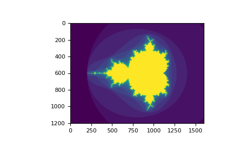
The second mode of indexing with booleans is more similar to integer indexing; for each dimension of the assortment we give a 1D boolean array selecting the slices we desire:

                                >>>                                a                =                np                .                arange                (                12                )                .                reshape                (                iii                ,                4                )                >>>                                b1                =                np                .                assortment                ([                Fake                ,                True                ,                True                ])                # first dim selection                >>>                                b2                =                np                .                array                ([                True                ,                Imitation                ,                True                ,                False                ])                # second dim pick                >>>                >>>                                a                [                b1                ,                :]                # selecting rows                array([[ 4,  5,  6,  7],                                  [ 8,  9, 10, 11]])                >>>                >>>                                a                [                b1                ]                # same thing                array([[ 4,  5,  6,  7],                                  [ 8,  ix, x, 11]])                >>>                >>>                                a                [:,                b2                ]                # selecting columns                array([[ 0,  two],                                  [ 4,  half-dozen],                                  [ eight, 10]])                >>>                >>>                                a                [                b1                ,                b2                ]                # a weird thing to do                array([ four, ten])              

Note that the length of the 1D boolean array must coincide with the length of the dimension (or centrality) yous want to piece. In the previous example, b1 has length 3 (the number of rows in a ), and b2 (of length 4) is suitable to alphabetize the second axis (columns) of a .

The ix_() function

The ix_ function tin be used to combine different vectors so as to obtain the result for each n-uplet. For case, if y'all want to compute all the a+b*c for all the triplets taken from each of the vectors a, b and c:

                                >>>                                a                =                np                .                array                ([                two                ,                iii                ,                four                ,                5                ])                >>>                                b                =                np                .                assortment                ([                viii                ,                five                ,                iv                ])                >>>                                c                =                np                .                array                ([                v                ,                4                ,                half dozen                ,                8                ,                three                ])                >>>                                ax                ,                bx                ,                cx                =                np                .                ix_                (                a                ,                b                ,                c                )                >>>                                ax                assortment([[[two]],                                  [[3]],                                  [[4]],                                  [[5]]])                >>>                                bx                assortment([[[eight],                                  [5],                                  [four]]])                >>>                                cx                array([[[5, four, 6, viii, 3]]])                >>>                                ax                .                shape                ,                bx                .                shape                ,                cx                .                shape                ((iv, 1, 1), (one, 3, 1), (one, 1, five))                >>>                                issue                =                ax                +                bx                *                cx                >>>                                result                array([[[42, 34, l, 66, 26],                                  [27, 22, 32, 42, 17],                                  [22, 18, 26, 34, 14]],                                  [[43, 35, 51, 67, 27],                                  [28, 23, 33, 43, 18],                                  [23, nineteen, 27, 35, fifteen]],                                  [[44, 36, 52, 68, 28],                                  [29, 24, 34, 44, nineteen],                                  [24, twenty, 28, 36, sixteen]],                                  [[45, 37, 53, 69, 29],                                  [30, 25, 35, 45, 20],                                  [25, 21, 29, 37, 17]]])                >>>                                result                [                3                ,                2                ,                iv                ]                17                >>>                                a                [                three                ]                +                b                [                2                ]                *                c                [                four                ]                17              

You could also implement the reduce equally follows:

                                >>>                                def                ufunc_reduce                (                ufct                ,                *                vectors                ):                ...                                vs                =                np                .                ix_                (                *                vectors                )                ...                                r                =                ufct                .                identity                ...                                for                five                in                vs                :                ...                                r                =                ufct                (                r                ,                v                )                ...                                return                r              

and and then utilize it equally:

                                >>>                                ufunc_reduce                (                np                .                add                ,                a                ,                b                ,                c                )                array([[[fifteen, xiv, 16, 18, thirteen],                                  [12, 11, 13, xv, x],                                  [11, ten, 12, 14,  9]],                                  [[16, 15, 17, xix, fourteen],                                  [13, 12, xiv, xvi, 11],                                  [12, xi, 13, 15, 10]],                                  [[17, 16, eighteen, twenty, 15],                                  [14, thirteen, 15, 17, 12],                                  [13, 12, xiv, 16, eleven]],                                  [[18, 17, 19, 21, 16],                                  [fifteen, fourteen, 16, 18, 13],                                  [14, thirteen, fifteen, 17, 12]]])              

The advantage of this version of reduce compared to the normal ufunc.reduce is that it makes utilize of the broadcasting rules in club to avert creating an statement array the size of the output times the number of vectors.

Indexing with strings

Run across Structured arrays.

Tricks and Tips

Here we give a listing of brusque and useful tips.

"Automatic" Reshaping

To change the dimensions of an array, you can omit ane of the sizes which will so be deduced automatically:

                                >>>                                a                =                np                .                arange                (                thirty                )                >>>                                b                =                a                .                reshape                ((                2                ,                -                1                ,                three                ))                # -1 means "any is needed"                >>>                                b                .                shape                (two, 5, iii)                >>>                                b                array([[[ 0,  i,  2],                                  [ 3,  iv,  5],                                  [ half-dozen,  7,  eight],                                  [ 9, 10, 11],                                  [12, thirteen, fourteen]],                                  [[15, xvi, 17],                                  [eighteen, 19, 20],                                  [21, 22, 23],                                  [24, 25, 26],                                  [27, 28, 29]]])              

Vector Stacking

How do we construct a 2D assortment from a list of equally-sized row vectors? In MATLAB this is quite easy: if x and y are two vectors of the same length you only need do 1000=[x;y] . In NumPy this works via the functions column_stack , dstack , hstack and vstack , depending on the dimension in which the stacking is to be washed. For example:

                                >>>                                x                =                np                .                arange                (                0                ,                10                ,                2                )                >>>                                y                =                np                .                arange                (                5                )                >>>                                m                =                np                .                vstack                ([                ten                ,                y                ])                >>>                                m                array([[0, ii, iv, 6, 8],                                  [0, i, 2, iii, 4]])                >>>                                xy                =                np                .                hstack                ([                x                ,                y                ])                >>>                                xy                array([0, 2, 4, 6, viii, 0, i, 2, 3, 4])              

The logic behind those functions in more than than two dimensions can be strange.

Histograms

The NumPy histogram function applied to an array returns a pair of vectors: the histogram of the assortment and a vector of the bin edges. Beware: matplotlib as well has a office to build histograms (called hist , as in Matlab) that differs from the one in NumPy. The main divergence is that pylab.hist plots the histogram automatically, while numpy.histogram simply generates the data.

                                >>>                                import                numpy                as                np                >>>                                rg                =                np                .                random                .                default_rng                (                one                )                >>>                                import                matplotlib.pyplot                as                plt                >>>                                # Build a vector of 10000 normal deviates with variance 0.5^2 and mean ii                >>>                                mu                ,                sigma                =                2                ,                0.five                >>>                                five                =                rg                .                normal                (                mu                ,                sigma                ,                10000                )                >>>                                # Plot a normalized histogram with fifty bins                >>>                                plt                .                hist                (                v                ,                bins                =                l                ,                density                =                Truthful                )                # matplotlib version (plot)                (array...)                >>>                                # Compute the histogram with numpy and and so plot it                >>>                                (                n                ,                bins                )                =                np                .                histogram                (                5                ,                bins                =                50                ,                density                =                Truthful                )                # NumPy version (no plot)                >>>                                plt                .                plot                (                .five                *                (                bins                [                1                :]                +                bins                [:                -                one                ]),                n                )              
../_images/quickstart-2.png

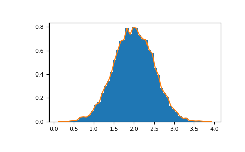
With Matplotlib >=3.4 you can also use plt.stairs(n, bins) .

Further reading

  • The Python tutorial

  • NumPy Reference

  • SciPy Tutorial

  • SciPy Lecture Notes

  • A matlab, R, IDL, NumPy/SciPy dictionary

  • tutorial-svd

sheadstakinan.blogspot.com

Source: https://numpy.org/devdocs/user/quickstart.html

0 Response to "Reading in Numpy Changes the Name of My Path"

Post a Comment

Iklan Atas Artikel

Iklan Tengah Artikel 1

Iklan Tengah Artikel 2

Iklan Bawah Artikel